Data Analysis - Correlation

Definition

Correlation measures the relationship between variables. In other words, it is a measure of how things are related and the process is called correlation analysis.

eg) Your caloric intake and your weight (high correlation)
A dog’s name and the type of dog food they prefer (low correlation)

Correlations are useful in that they can let us make predictions about future behaviour of things.

The Correlation Coefficient

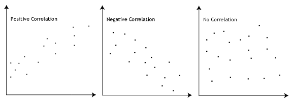
A correlation coefficient quantifies the relationship, ranging from -1 to 1.

0 means there is no relationship -1 or 1 means that there is a perfect negative or positive correlation

Specifically, a positive correlation means that as the value of one variable increases, so does the value of the other variable. A negative correlation means that as the value of one variable increases, the value of the other variable decreases.

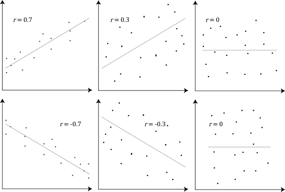
In particular, Pearson correlation coefficient is a measure of the strength of a linear relationship between two variables denoted by r. Pearson correlation tries to draw a line of best fit through the data of two variables and r represents how far away the data points are from thie line of best fit. (i.e. how well the data points fit this model/line)

Strength of association

If the Pearson coefficient r is close to 1 or -1, that means the association of the two variables is stronger. If r is 1 or -1, that implies that all our data points are included on the line of best fit. (no variation exists) The closer the value of r to 0, the greater the variation around the line of best fit.

Some examples are shown below.

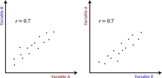
NOTE: The Pearson coefficient makes no account of any logic behind why or how we chose the two variables to compare, meaning that it doesn’t matter which is dependent on the other. All variables are treated equally. For example, we can plot a graph of basketball performance against height and say r comes out to be 0.76. This means that as height increases, so does the performance. But if we plotted the graph the other way around, we would still get r = 0.76.

Assumptions made by Pearson’s Correlation Test

In many cases when working with real-world data which is often “messy”, Perason’s correlation will not be suitable statistical test to use because the data doesn’t meet one or more of the seven assumptions made by the test. Thus, the solution is to use a different statistical test or make adjustments to our data.

• Assumption 1: The two variables should be measured on a continous scale. (i.e. measured at the interval or ratio level) For example, revision time (measured in hours), intelligence (measured using IQ score), exam score (measured from 0 to 100), etc.

• Assumption 2: The two continuous variables should be paired such that each case has two values, one for each variable. For example, if we have two variables “revision time” and “exam score” and sampled 100 students at a university, each of the 100 students(cases) would have a value for revision time and an exam result.

• Assumption 3: There should be independence of cases, which means that student #1 case should be independent of any other cases(student #2, student #50, etc.) If they are not independent, they are related, and Pearson’s correlation is not an appropriate statistical test.
  
  For example, if some of the 100 students were in a study group, we can expect the relationship between revision time and exam score for the students in that group to be more similar when compared to others, violating the independence of cases assumption. So there shouldn’t be an extra variable or setting that connects two cases.

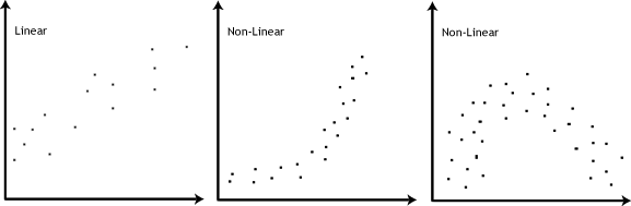
• Assumption 4: There should be a linear relationship between your two continouous variables. To test this, simply plot them on a graph (eg. scatterplot) and visually inspect the graph’s shape. It is not appropriate to analyse a non-linear relationship using Pearson correlation.

• Assumption 5: Theoretically, both continuous variables should follow a bivariate normal distribution. However, in practice, it is usually accepted that having univariate normality in both variables is sufficient. (i.e. each variable is normally distributes)
  
  Hence, if one or both variables is not normally distributed, then there is disagreement about whether Pearson’s correlation will provide a valid result. In this case, there are more robust methods that can be considered instead. (see Shevlyakov and Oja, 2016)

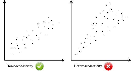
• Assumption 6: There should be homoscedasticity, which means that the variances along the line of best fit remain similar as you move along the line. If not, then there is heteroscedasticity. We can see the comparison below.

• Assumption 7: There should be no univariate or multivariate outliers. In other words, we need to consider outliers that are unusual only on one variable (univariate outliers), as well as those that are an unusual “combination” of both variables (multivariate outliers).
  
  Taking the same example as above, if all students scored between 45% and 95% except for one who scored a very low 5% in their exam, this individual would be a univariate outlier. That is, they have an unusual score for this specific variable irrespective of the values ot the other variable. (i.e. revision time)
  
  Now, let’s assume that the revision time is positively correlated with exam score. If a student did almost no studying, but aced the exam, they would be a multivariate outlier and vice versa. Basically, a multivariate outlier is an outlier that “bucks the trend” of the data.

출처: https://statistics.laerd.com/statistical-guides/pearson-correlation-coefficient-statistical-guide.php